Parallel Data Processing
| Graph Allocation |
| Component Allocation |
| Partitioning/Gathering Data |
| Node Allocation Limitations |
| Sandboxes in Cluster |
| Using a Sandbox Resource as a Component Data Source |
This type of scalability is currently only available for Graphs. Jobflow and Profiler jobs cannot run in parallel.
When a transformation is processed in parallel, the whole graph (or its parts) runs in parallel on multiple Cluster nodes having each node process just a part of the data. The data may be split (partitioned) before the graph execution or by the graph itself on the fly. The resulting data may be stored in partitions or gathered and stored as one group of data.
Ideally, the more nodes we have in a Cluster, the more data can be processed in a specified time. However, if there is a single data source which cannot be read by multiple readers in parallel, the speed of further data transformation is limited. In such cases, parallel data processing is not beneficial since the transformation would have to wait for input data.
Graph Allocation
Each graph executed in a Clustered environment is automatically subjected to a transformation analysis. The object of this analysis is to find a graph allocation. The graph allocation is a set of instructions defining how the transformation should be executed:
First of all, the analysis finds an allocation for individual components. The component allocation is a set of Cluster nodes where the component should be running. There are several ways how the component allocation can be specified (see the following section), but a component can be requested to run in multiple instances. In the next step an optimal graph decomposition is decided to ensure all component allocation will be satisfied, and the number of remote edges between graph instances is minimized.
Resulted analysis shows how many instances (workers) of the graph need to be executed, on which Cluster nodes they will be running and which components will be present in them. In other words, one executed graph can run in many instances, each instance can be processed on an arbitrary Cluster node and each contains only convenient components.
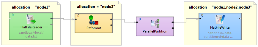
Figure 42.1. Component allocations example
This figure shows a sample graph with components with various allocations.
FlatFileReader: node1
Reformat: node2
FlatFileWriter: node1, node2 and node3
ParallelPartition can change cardinality of allocation of two interconnected components (detailed description of Cluster partitioning and gathering follows this section).
Visualization of the transformation analysis is shown in the following figure:
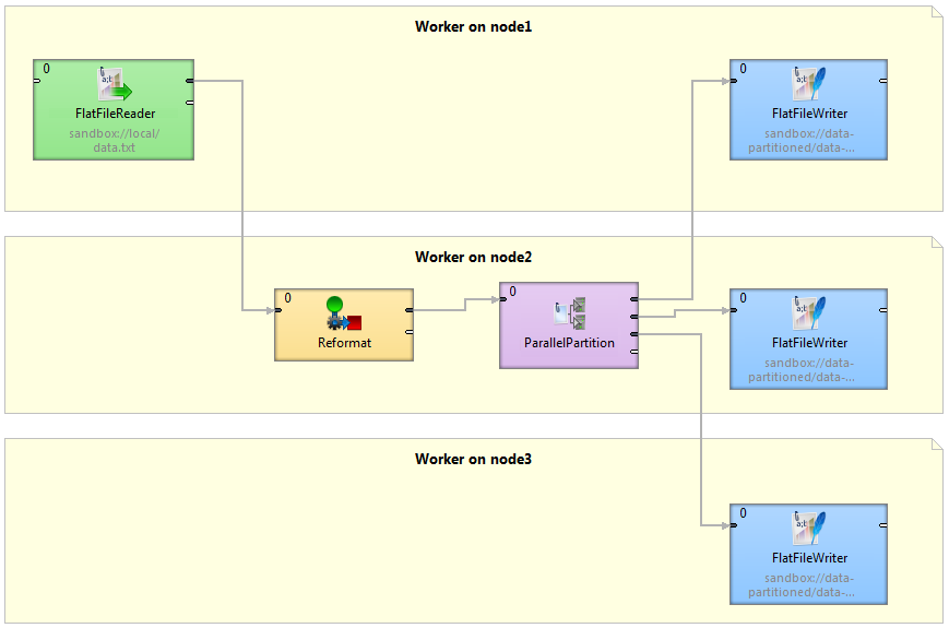
Figure 42.2. Graph decomposition based on component allocations
Three workers (graphs) will be executed, each on a different Cluster node. Worker on Cluster node1 contains FlatFileReader and first of three instances of the FlatFileWriter component. Both components are connected by remote edges with components which are running on node2. The worker running on node3 contains FlatFileWriter fed by data remotely transferred from ParallelPartitioner running on node2.
Component Allocation
Allocation of a single component can be derived in several ways (list is ordered according to priority):
Explicit definition - all components have a common attribute Allocation:
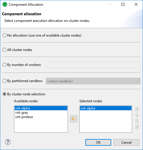
Figure 42.3. Component allocation dialog
Three different approaches are available for explicit allocation definition:
Allocation based on the number of workers - the component will be executed in requested instances on some Cluster nodes which are preferred by CloverDX Cluster. Server can use a build-in load balancing algorithm to ensure the fastest data processing.
Allocation based on reference on a partitioned sandbox - component allocation corresponds with locations of given partitioned sandbox. Each partitioned sandbox has a list of locations, each bound to a specific Cluster node. Thus allocation would be equivalent to the list of locations. For more information, see Partitioned sandbox in Sandboxes in Cluster.
Allocation defined by a list of Cluster node identifiers (a single Cluster node can be used more times)
Reference to a partitioned sandbox FlatFileReader, FlatFileWriter and ParallelReader components derive their allocation from the
fileURLattribute. In case the URL refers to a file in a partitioned sandbox, the component allocation is automatically derived from locations of the partitioned sandbox. So in case you manipulate with one of these components with a file in partitioned sandbox, a suitable allocation is used automatically.Adoption from neighbor components By default, allocation is inherited from neighbor components. Components on the left side have a higher priority. Cluster partitioners and Cluster gathers are nature bounds for recursive allocation inheritance.
Partitioning/Gathering Data
As mentioned before, data may be partitioned and gathered in several ways:
Partitioning/gathering "on the fly"
There are six special components to consider: ParallelPartition, ParallelLoadBalancingPartition, ParallelSimpleCopy, ParallelSimpleGather, ParallelMerge, ParallelRepartition. They work similarly to their non-Cluster variations, but their splitting or gathering nature is used to change data flow allocation, so they may be used to change distribution of the data among workers.
ParallelPartition and ParallelLoadBalancingPartition work similar to a common partitioner - they change the data allocation from 1 to N. The component preceding the ParallelPartitioner runs on just one node, whereas the component behind the ParallelPartitioner runs in parallel according to node allocation.
ParallelSimpleCopy can be used in similar locations. This component does not distribute the data records, but copies them to all output workers.
ParallelSimpleGather and ParallelMerge work in the opposite way. They change the data allocation from N to 1. The component preceding the gather/merge runs in parallel while the component behind the gather runs on just one node.
Partitioning/gathering data by external tools
Partitioning data on the fly may in some cases be an unnecessary bottleneck. Splitting data using low-level tools can be much better for scalability. The optimal case being that each running worker reads data from an independent data source, so there is no need for a ParallelPartitioner component, and the graph runs in parallel from the beginning.
Or the whole graph may run in parallel, however the results would be partitioned.
Node Allocation Limitations
As described above, each component may have its own node allocation specified, which may result in conflicts.
Node allocation of neighboring components must have the same cardinality.
It does not have to be the same allocation, but the cardinality must be the same. For example, there is a graph with 2 components: DataGenerator and Trash.
DataGenerator allocated on NodeA sending data to Trash allocated on NodeB works.
DataGenerator allocated on NodeA sending data to Trash allocated on NodeA and NodeB fails.
Node allocation behind the ParallelGather and ParallelMerge must have cardinality 1.
It may be of any allocation, but the cardinality must be just 1.
Node allocation of components in front of the ParallelPartition, ParallelLoadBalancingPartition and ParallelSimpleCopy must have cardinality 1.
Sandboxes in Cluster
There are three sandbox types in total - shared sandboxes, and partitioned and local sandboxes (introduced in 3.0) which are vital for parallel data processing.
Shared Sandbox
This type of sandbox must be used for all data which is supposed to be accessible on all Cluster nodes. This includes all graphs, jobflows, metadata, connections, classes and input/output data for graphs which should support HA. All shared sandboxes reside in the directory, which must be properly shared among all Cluster nodes. You can use a suitable sharing/replicating tool according to the operating system and filesystem.
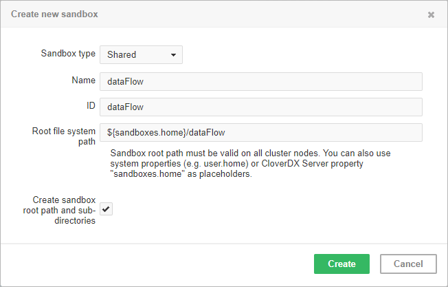
Figure 42.4. Dialog form for creating a new shared sandbox
As you can see in the screenshot above,
you can specify the root path on the filesystem and you can use a placeholders or absolute path.
Placeholders available are environment variables, system properties or
CloverDX Server configuration property intended for this use: sandboxes.home.
Default path is set as [user.data.home]/CloverDX/sandboxes/[sandboxID]
where the sandboxID is an ID specified by the user.
The user.data.home placeholder refers to the home directory of the user running the JVM process
(/home subdirectory on Unix-like OS);
it is determined as the first writable directory selected from the following values:
USERPROFILEenvironment variable on Windows OSuser.homesystem property (user home directory)user.dirsystem property (JVM process working directory)java.io.tmpdirsystem property (JVM process temporary directory)
Note that the path must be valid on all Cluster nodes. Not just nodes currently connected to the Cluster, but also on nodes that may be connected later. Thus when the placeholders are resolved on a node, the path must exist on the node and it must be readable/writable for the JVM process.
Local Sandbox
This sandbox type is intended for data, which is accessible only by certain Cluster nodes. It may include massive input/output files. The purpose being, that any Cluster node may access content of this type of sandbox, but only one has local (fast) access, and this node must be up and running to provide data. The graph may use resources from multiple sandboxes which are physically stored on different nodes, since Cluster nodes are able to create network streams transparently as if the resources were a local file. For details, see Using a Sandbox Resource as a Component Data Source.
Do not use a local sandbox for common project data (graphs, metadata, connections, lookups, properties files, etc.). It would cause odd behavior. Use shared sandboxes instead.
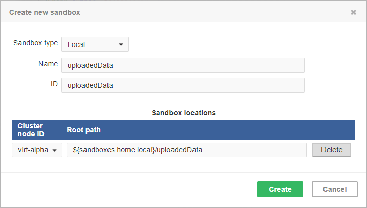
Figure 42.5. Dialog form for creating a new local sandbox
The sandbox location path is pre-filled with the sandboxes.home.local placeholder
which, by default, points to [user.data.home]/CloverDX/sandboxes-local.
The placeholder can be configured as any other CloverDX configuration property.
Partitioned Sandbox
This type of sandbox is an abstract wrapper for physical locations existing typically on different Cluster nodes. However, there may be multiple locations on the same node. A partitioned sandbox has two purposes related to parallel data processing:
node allocation specification
Locations of a partitioned sandbox define the workers which will run the graph or its parts. Each physical location causes a single worker to run without the need to store any data on its location. In other words, it tells the CloverDX Server: to execute this part of the graph in parallel on these nodes.
storage for part of the data
During parallel data processing, each physical location contains only part of the data. Typically, input data is split in more input files, so each file is put into a different location and each worker processes its own file.
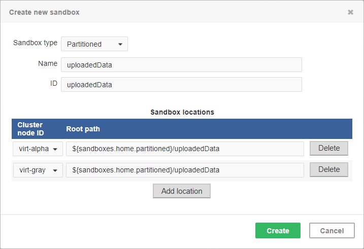
Figure 42.6. Dialog form for creating a new partitioned sandbox
As you can see on the screenshot above, for a partitioned sandbox, you can specify one or more physical locations on different Cluster nodes.
The sandbox location path is pre-filled with the sandboxes.home.partitioned placeholder
which, by default, points to [user.data.home]/CloverDX/sandboxes-partitioned.
The sandboxes.home.partitioned config property may be configured
as any other CloverDX Server configuration property.
Note that the directory must be readable/writable for the user running JVM process.
Do not use a partitioned sandbox for common project data (graphs, metadata, connections, lookups, properties files, etc.). It would cause odd behavior. Use shared sandboxes instead.
Using a Sandbox Resource as a Component Data Source
A sandbox resource, whether it is a shared, local or partitioned sandbox (or ordinary sandbox on standalone server), is specified in the graph under the fileURL attributes as a so called sandbox URL like this:
sandbox://data/path/to/file/file.dat
where data is a code for the sandbox and path/to/file/file.dat
is the path to the resource from the sandbox root.
The URL is evaluated by CloverDX Server during job execution,
and a component (reader or writer) obtains the opened stream from the Server.
This may be a stream to a local file or to some other remote resource.
So a job does not have to run on the node which has local access to the resource.
There may be more sandbox resources used in the job, and each of them may be on a different node.
The sandbox URL has a specific use for parallel data processing. When the sandbox URL with the resource in a partitioned sandbox is used, that part of the graph/phase runs in parallel, according to the node allocation specified by the list of partitioned sandbox locations. Thus, each worker has it is own local sandbox resource. CloverDX Server evaluates the sandbox URL on each worker and provides an open stream to a local resource to the component.
The sandbox URL may be used on the standalone Server as well. It is suitable for graphs referencing resources from different sandboxes. It may be metadata, lookup definition or input/output data. A referenced sandbox must be accessible for the user who executes the graph.