Example of Distributed Execution
| Details of the Example Transformation Design |
| Scalability of the Example Transformation |
The following diagram shows a transformation graph used for parsing invoices generated by cell phone network providers.
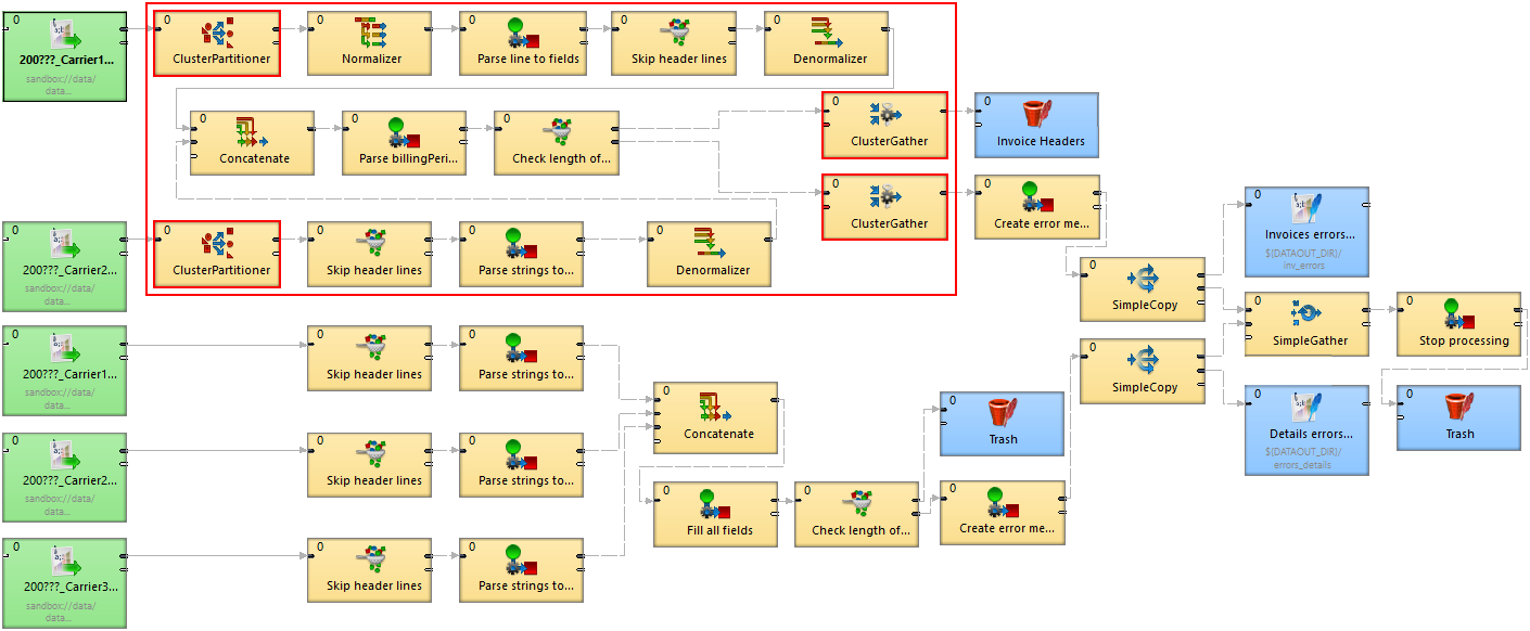
The size of these input files may be up to a few gigabytes, so it is very beneficial to design the graph to work in Cluster environment.
Details of the Example Transformation Design
Note there are four Cluster components in the graph and these components define a point of "node allocation" change, so the part of the graph demarcated by these components is highlighted by the red rectangle. The allocation of these components should be performed in parallel. This means that the components inside the rectangle should have convenient allocation. The rest of the graph runs on a single node.
Specification of "node allocation"
There are 2 node allocations used in the graph:
node allocation for components running in parallel (demarcated by the four Cluster components)
node allocation for the outer part of the graph which runs on a single node
The single node is specified by the sandbox code used in the URLs of input data.
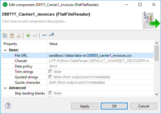
The following dialog shows the File URL value:
sandbox://data/path-to-csv-file,
where data is the ID of the server sandbox containing the specified file.
And it is the data local sandbox which defines the single node.
The part of the graph demarcated by the four Cluster components may have specified its allocation by the file URL attribute as well, but this part does not work with files at all, so there is no file URL. Thus, we will use the node allocation attribute. Since components may adopt the allocation from their neighbors, it is sufficient to set it only for one component.
Again, dataPartitioned in the following dialog is the sandbox ID.
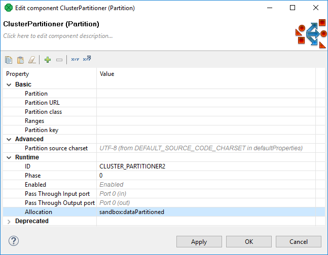
This project requires 3 sandboxes: data, dataPartitioned and PhoneChargesDistributed.
data
contains input and output data
local sandbox (yellow folder), so it has only one physical location
accessible only on node
i-4cc9733bin the specified path
dataPartitioned
partitioned sandbox (red folder), so it has a list of physical locations on different nodes
does not contain any data and since the graph does not read or write to this sandbox, it is used only for the definition of "nodes allocation"
on the following figure, the allocation is configured for two Cluster nodes
PhoneChargesDistributed
common sandbox containing the graph file, metadata, and connections
shared sandbox (blue folder), so all Cluster nodes have access to the same files
If the graph was executed with the sandbox configuration of the previous figure, the node allocation would be:
components which run only on a single node, will run only on the
i-4cc9733bnode according to the "data" sandbox location.components with an allocation according to the dataPartitioned sandbox will run on nodes
i-4cc9733bandi-52d05425.
Scalability of the Example Transformation
The example transformation has been tested in an Amazon Cloud environment with the following conditions for all executions:
the same master node
the same input data: 1.2GB of input data, 27 million records
three executions for each "node allocation"
"node allocation" changed between every 2 executions
all nodes has been of "c1.medium" type
We tested "node allocation" cardinality from 1 single node, all the way up to 8 nodes.
The following figure shows the functional dependence of run-time on the number of nodes in the Cluster:
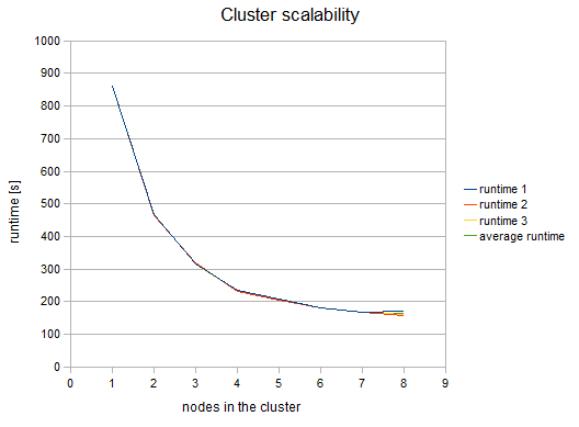
Figure 42.7. Cluster Scalability
The following figure shows the dependency of a speedup factor on the number of nodes in the Cluster. The speedup factor is the ratio of the average runtime with one Cluster node and the average runtime with x Cluster nodes. Thus:
speedupFactor = avgRuntime(1 node) / avgRuntime(x nodes)
We can see, that the results are favorable up to 4 nodes. Each additional node still improves the Cluster performance; however, the effect of the improvement decreases. Nine or more nodes in the Cluster may even have a negative effect because their benefit for performance may be lost in the overhead with the management of these nodes.
These results are specific for each transformation, there may be a transformation with a much better or possibly worse function curve.
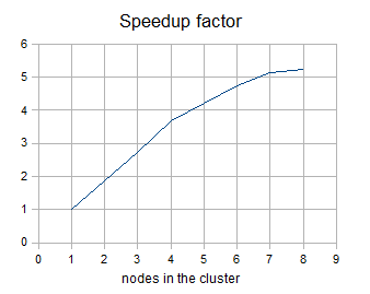
Figure 42.8. Speedup factor
Table of measured runtimes:
| nodes | runtime 1 [s] | runtime 2 [s] | runtime 3 [s] | average runtime [s] | speedup factor |
|---|---|---|---|---|---|
| 1 | 861 | 861 | 861 | 861 | 1 |
| 2 | 467 | 465 | 466 | 466 | 1.85 |
| 3 | 317 | 319 | 314 | 316.67 | 2.72 |
| 4 | 236 | 233 | 233 | 234 | 3.68 |
| 5 | 208 | 204 | 204 | 205.33 | 4.19 |
| 6 | 181 | 182 | 182 | 181.67 | 4.74 |
| 7 | 168 | 168 | 168 | 168 | 5.13 |
| 8 | 172 | 159 | 162 | 164.33 | 5.24 |