
Version
ProfilerProbe
Licensed under CloverDX Data Quality package.
Short Description
ProfilerProbe analyses (profiles) input data. The big advantage of the component is the combined power of CloverDX solutions with data profiling features. So it makes profiling accessible in very complex workflows such as data integration, data cleansing and other processing tasks.
ProfilerProbe is not limited to only profiling isolated data sources; instead, it can be used for profiling data from various sources (including popular DBs, flat files, spreadsheets etc.). ProfilerProbe is capable of handling all data sources supported by CloverDX's Readers.
|
To be able to use this component, you need a separate Data Quality license. |
| Component | Same input metadata | Sorted inputs | Inputs | Outputs | Each to all outputs | Java | CTL | Auto-propagated metadata |
|---|---|---|---|---|---|---|---|---|
ProfilerProbe |
- |
⨯ |
1 |
1-n |
✓ |
⨯ |
⨯ |
✓ |
Ports
| Port type | Number | Required | Description | Metadata |
|---|---|---|---|---|
Input |
0 |
✓ |
Input data records to be analyzed by metrics. |
Any |
Output |
0 |
⨯ |
A copy of input data records. |
Input port 0 |
1-n |
⨯ |
Results of data profiling per individual field. |
Any |
Metadata
ProfilerProbe propagates metadata from the first input port to the first output port and from the first output port to the first input port.
ProfilerProbe does not change the priority of propagated metadata.
If any metric is set up in the component, the component has a template ProfilerProbe_RunResults on its second output port. The field names and data types depend on used metrics.
ProfilerProbe Attributes
| Attribute | Req | Description | Possible values |
|---|---|---|---|
Basic |
|||
Metrics |
✓ |
Statistics you want to be calculated on metadata fields. Learn more about metrics in Metrics section. |
See List of Metrics. |
Output mapping |
Maps profiling results to output ports, starting from port number 1. See Details. |
||
Advanced |
|||
Output mapping URL |
External XML file containing the Output mapping definition. |
||
Processing mode |
|
Always active (default) | Debug mode only |
|
Details
ProfilerProbe calculates metrics of the data that is coming through its first input port. You can choose which metrics you want to apply on each field of the input metadata. You can use this component as a 'probe on an edge' to get a more detailed (statistical) view of data that is flowing in your graph.
The component sends an exact copy of the input data to output port 0 (behaves as SimpleCopy). That means you can use ProfilerProbe in your graphs to examine data flowing in it, without affecting the graph’s business logic itself.
The remaining output ports contain results of profiling, i.e. metric values for individual fields.
Output mapping
Editing the Output mapping attribute opens the Transform Editor where you can decide which metrics to send to output ports.
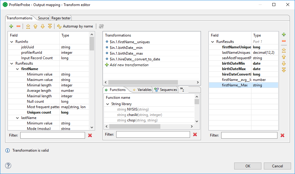
Figure 420. Transform Editor in ProfilerProbe
The dialog provides you with all the power and features known from Transform Editor and CTL.
In addition, notice metadata on the left hand side has a special format.
It is a tree of input fields AND metrics you assigned to them via the Metrics attribute.
Fields and metrics are grouped under the RunResults record.
Each field in RunResults record has a special name: fieldNamemetric_name (note the underscore is doubled as a separator), e.g. firstNameavg_length.
Additionally there is another special record containing three fields - JobUid, inputRecordCount and profilerRunId.
After you run your graph, the field will store the total number of records which were profiled by the component.
You can right-click a field/metric and Expand All, or Collapse All metrics.
To do the mapping in a few basic steps, follow these instructions:
-
Provided you already have some output metadata, just left-click a metric in the left-hand pane and drag it onto an output field. This will send profiling results of that particular metric to the output.
-
If you do not have any output metadata:
-
Drag a Field from the left hand side pane and drop it into the right hand pane (an empty space).
-
This produces a new field in the output metadata. Its format is:
fieldNamemetric_name(note the underscore is doubled as a separator), e.g.firstNameavg_length. -
You can map metrics to fields of any output port, except for port 0. That port is reserved for input data (which just flows through the component without being affected in the process).
-
|
The output mapping uses CTL (you can switch to the Source tab). All kinds of functions are available to help you learn even more about your data, for example: calculates the per cent of unique first names in all records. |
If you do not define the output mapping, the default output mapping is used:
$out.0.* = $in.0.*;The default output mapping is available since version 4.1.0.
Importing metrics
In the Metrics dialog, you can import your settings of fields and their metrics from a *.cpj file using the Import from .cpj button at the bottom of the dialog.
The purpose of the import is for easier transition from previous versions, it is no longer possible to externalize metrics to a *.cpj file.
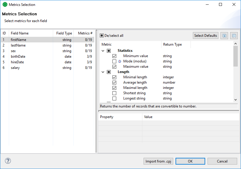
Figure 421. Import metrics button
ProfilerProbe Notes & Limitations
-
If you want to use sampling of the input data, connect the DataSampler (or other filter) component to your graph. There is no built-in sampling in ProfilerProbe.
-
In Cluster environment, the component will profile data from each node where it is running. Therefore, the results are only applicable to the portions of data processed on given node. If you need to compute metrics for data from all nodes, first gather the data to single node where this component will run (e.g. by using ParallelSimpleGather).
Compatibility
| Version | Compatibility Notice |
|---|---|
4.1.0 |
Default mapping is now available. |
Troubleshooting
The ProfilerProbe component can report an error similar to:
CTL code compilation finished with 1 errors
Error: Line 5 column 23 - Line 5 column 39: Field 'field1__avg_length' does not exist in record 'RunResults'!
This means that you’re accessing a disabled metric in output mapping - in this example the Average length is not enabled on the field field1.
Metrics
The major goal when setting up ProfilerProbe component is to select metrics that will be calculated for each metadata field.
First select a field on the left hand side and second check metrics on the right hand side. Some metrics are selected by default.
The range of available metrics differs for each field and depends on Field Type. Thus, you can analyze e.g. the average value or median for integers while in strings, you can measure the shortest string, non-ASCII records and so forth.
In addition, you can work with more fields at a time by selecting them (Ctrl+click, Shift+click) and assigning metrics to the whole group.
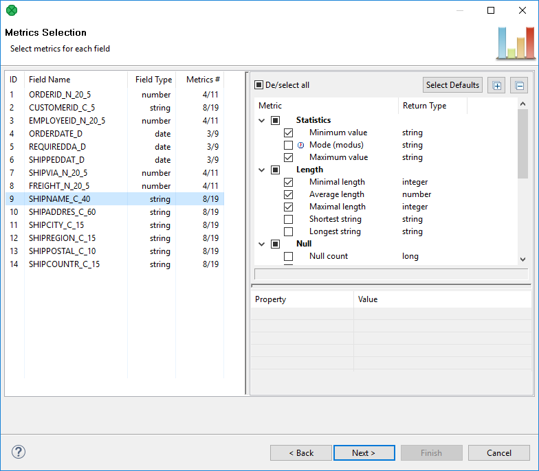
Figure 422. Selecting and configuring metrics
Some metrics just need to be checked while some others require additional settings.
If a metric is checked and can actually be configured, you will notice the Property | Value area in the bottom right hand corner becomes active. An example of one such metric is Time unit chart, see the following picture.
Some metrics return map or list data types. Such metrics have their return type marked with an icon, see Most frequent patterns and Non printable ASCII in the picture above.
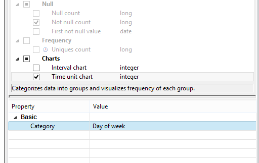
Figure 423. Metric configuration. Note the metric has to be checked.
List of Metrics
| Metric | Return type | Description | Note |
|---|---|---|---|
Statistics |
|||
Minimum value |
number / string |
Returns the lowest value of all numbers. The metric works with strings, too. Example: let us have two strings, "zoo" and "city-zoo". The second one is Minimum value, because alphabetically, it would be the first item of the two. |
|
Average value |
number |
Calculates the average value of all numbers. |
|
Median |
number |
Calculates the median of your data. Be advised that profiling huge data sets with this metric works slower (the reason is necessary values are continually stored in the database until the median is finally calculated). |
|
Mode (modus) |
string |
Returns the value which is most frequently repeated in the data set. Be advised that profiling huge data sets with this metric works slower (the reason is necessary values are continually stored in the memory until modus is finally calculated). |
|
Maximum value |
number / string |
Returns the highest value of all numbers. The metric works with strings, too. Example: let us have two strings, "zoo" and "city-zoo". The first one is Maximum value, because alphabetically, it would be the last item of the two. |
|
Length |
|||
Minimal length |
integer |
Examines the data set and returns the length of the string consisting of the lowest number of characters. |
|
Average length |
number |
Calculates the average length of all field values. |
|
Maximal length |
integer |
Examines the data set and returns the length of the string consisting of the highest number of characters. |
|
Shortest string |
string |
Returns the shortest found string of the data set. If there are more of them, the first one alphabetically is returned. |
|
Longest string |
string |
Returns the longest found string of the data set. If there are more of them, the last one alphabetically is returned. |
|
Null Handling |
|||
Null count |
integer |
Returns the count of values that are |
|
Not null count |
integer |
Counts all fields that carry some data, i.e. they are not |
|
First not null value |
string |
Returns the first value found which is not null. |
|
String format |
|||
Most frequent patterns |
string |
The metric examines all strings and returns a mask that describes how those strings most commonly look like. You can configure the number of returned patterns via Patterns count. Example result: "27,1%: A99 9AA 9,2%: AA9 5,8%: 999" - it tells you that 27,1% of strings looked like "A99 9AA", 9,2% were "AA9" and 5,8% were "999" where A stands for an arbitrary character and 9 is a digit. One such "A99 9AA" string could be e.g. "M64 1se". Profiling huge data sets with this metric may work slower if they contain "ugly" strings consisting of brackets, quotes, commas and other non-alphanumeric characters. |
This metric returns a map with keys containing patterns and values containing their occurrences. |
Least frequent patterns |
string |
The metric examines all strings and returns a mask that describes how those strings least commonly look like. You can configure the number of returned patterns via Patterns count. Example result: "5,8%: 999 9,2%: AA9 27,1%: A99 9AA " - it tells you that 5,8% of strings looked like "999", 9,2% were "AA9" and 27,1% were "A99 9AA" where A stands for an arbitrary character and 9 is a digit. One such "A99 9AA" string could be e.g. "M64 1se". Profiling huge data sets with this metric may work slower if they contain "ugly" strings consisting of brackets, quotes, commas and other non-alphanumeric characters. |
This metric returns a map with keys containing patterns and values containing their occurrences. |
Convertible to date |
integer |
The metric finds out how many records can be converted to a date format. The format you are looking for has to be specified in Mask. Setting the appropriate Locale allows the metric to e.g. recognize month names written as strings. |
|
Convertible to number |
integer |
The metric finds out how many records can be converted to a number. Optionally, type in the Format pattern you are looking for. The pattern uses the same syntax as CloverDX Designer (e.g. '0' for digit, '.' for decimal separator) - please refer to Numeric Format documentation. |
|
Non-ASCII records |
integer |
Returns the number of records containing non-ASCII characters. |
|
Non printable ASCII |
string |
Gets all ASCII characters that cannot be printed (e.g. Delete or Escape). |
This metric returns a list of the non printable ASCII characters. |
Frequency |
|||
Uniques count |
integer |
Returns the amount of values that are unique within the data set. Thus, you can e.g. easily pick a field which could serve as the primary key. Profiling huge data sets with this metric works slower as unique values are gradually stored in the memory. |
|
Interval chart |
chart |
A histogram chart showing values divided into interval bins with a number of occurrences per each value. It can be used for numerical (integer, long, double, decimal) and date fields. This metric can either work in an automatic mode (no configuration) or you can set its properties yourself. The automatic mode always sets the histogram so that all your data could be displayed. The number of buckets is chosen adequately. Thus, the automatic mode gets you a good overview of how your data is spread. Afterwards, you may want to focus on a certain part of the data. In that case, set histogram properties. Be advised you have to set all of them, otherwise the job will fail on running. The aforementioned properties differ for integer fields and date fields. As for integer fields, you set:
While for date fields, you set:
|
|
Frequency chart |
chart |
A simple chart showing the number of occurrences per each value. It can be used for strings and numerical fields (integer, long). Use it to analyze long listings, e.g. (postal) codes. You define the maximum number of unique values the metric will work with - Maximum unique values. If this threshold is exceeded during the computation, the histogram will not be shown. In case you are profiling a file with many unique values, the histogram will allow you to switch between the Most common and Least common ones. |
|
Time unit chart |
chart |
A special chart for 1900-01-02 12:34:56 2011-06-22 22:34:11 These would fit into the same bucket only if you chose Minute as Category. For all other categories, they would fall in different buckets. |
|